Related Pages:
Excuses offered for not worrying about receiver damage from close-spaced antennas:
I never saw or heard of this problem, so it is not a worry.
Fact: Outside of contests not too many of us have same-band antennas, or antennas with good harmonic response, that are connected to receivers and transmitters at the same time. It would be unreasonable to think anyone would commonly damage receivers because very few people have antennas that work well on the same band coupled to a receiver, while a transmitter is running.
Police, public service, and marine installations operate multiple radios without problems, so it should be the same for HF radios.
Fact: Power levels, for the same antenna spacings in feet, decrease decrease dramatically as frequency increases. A 3.5 MHz installation with 1/4 wave verticals has well over 100 times the coupled power of two 2-meter antennas, when both systems have the same physical spacing.
I can just turn the other radio off, or not tune it to the same frequency, and it will be safer.
Fact: Overload damage to nearly all radios is unaffected by the distance off frequency the radio is tuned. HF radios often are minimally affected by having power on or off, or the band they are on.
If you are using close-spaced antennas with multiple radios, especially with very close spacing or higher power, we should worry about damage. We should test the system to get at least some rough idea how significant coupled power is.
Coupled Power Levels, between transmitting and receiving antennas
People sometimes ask the safe minimum antenna spacing to avoid damage to radios. The data below should help prevent damage at Field Day or in other multiple transmitter contest or emergency operating environments. The data below is based on two matched antennas, where the load (the receiver) matches the antenna impedance. The systems have no feed line losses.
Data below does not represent an absolute maximum coupling. Levels can be higher, depending on antenna height and orientation. Levels can also be much less, but the levels below are a very reasonable estimate of maximum power for typical antenna installations.
Some basic rough rules for reasonably wide antenna spacings:
1.) Doubling spacing distance reduces power 2-4 times (at very wide spacings or far field with horizontal antennas, power diminishes quite rapidly).
2.) Outside of very close spacing, doubling frequency, with a fixed physical distance between antennas, reduces coupled power by about four times.
3.) A dipole and a vertical have minimum coupling when the vertical is centered on and directly broadside to the dipole. Coupling to a vertical actually increases off the dipole ends. If we want best isolation, we should not install a dipole or horizontal antenna with horizontal antenna ends toward the vertical.
4.) Two horizontal dipoles have minimal coupling when they are nearly end-to-end, but this varies with height and soil.
5.) Improper feed systems, such as those with common mode currents, can radically increase coupling levels between antennas.
6.) Some receivers are more damage prone than than others. Most receivers I've tested will handle over 20 dBm (100 mW or 1/10th of a watt) for extended periods without damage. Most newer receivers use 1/8th watt resistors in attenuator pads, and have other parts that can be damaged at 1 watt or so. I consider any receive antenna power over .125 watts to be potentially damaging to receivers, and over .5 watts to likely cause damage, but this is just my opinion.
7.) Damage problems are generally from same-band operation, not same frequency operation. Tuning off-frequency does not reduce chances of damage. The exact frequency difference between a transmitter and receiver does not matter much, but the band does. This is because the radio's wide bandpass filters pass the signal on to easily damaged components, which are ahead of the mixer and narrow selectivity.
8.) Turning a receiver off usually will not eliminate chances of overload damage, and often does not even reduce damage from high coupled power levels. If we don't want radio damage, we should disconnect the antenna from the unused receiver, or make sure coupling from the transmitter to the receiver is at safe levels.
9.) It is unlikely that transmitter or amplifier harmonics will damage receivers. Nearly all 1500-watt amplifiers have less than 50 milliwatts on the worse harmonic. While that level can travel thousands of miles, it is far below damaging levels at any distance. The real danger is an intentionally generated signal's fundamental energy getting into early receiver components.
Coupled Power Levels
The following levels are based on EZNEC models. The models use same-band antennas, which is a worse-case condition.
Two 1/4-wave verticals, each with zero ground loss. Transmitter power at antenna = 1000 watts
| Band | 400-foot spacing | 200-foot spacing | 100-foot spacing | 50-foot spacing | 25-foot spacing |
| 160 | 26 watts | 66 watts | 207 watts | ||
| 80 | 7.5 watts | 29 watts | 67.5 watts | 223 watts | |
| 40 | 2 watts | 7.5 watts | 29 watts | 67.5 watts | 223 watts |
| 20 | 0.5 watts | 2 watts | 7.5 watts | 29 watts | 67.5 watts |
| 10 | 0.125 watts | 0.5 watts | 2 watts | 7.5 watts | 29 watts |
Dipole-to-vertical that is broadside-to and centered-on the dipole, perfect ground,
and 1000 watts
| Band | 400-foot spacing | 200-foot spacing | 100-foot spacing | 50-foot spacing | 25-foot spacing |
| 160 | 0.13 watts | 0.38 watts | 0.79 watts | ||
| 80 | .049 watts | 0.13 watts | 0.38 watts | 0.79 watts | |
| 40 | .013 watts | .049 watts | 0.13 watts | 0.38 watts | 0.79 watts |
| 20 | .013 watts | .049 watts | 0.13 watts | 0.38 watts | |
| 10 | .013 watts | .049 watts | 0.13 watts |
Vertical-to-dipole, dipole oriented so vertical is nearly in line with the dipole's end
| Band | 400-foot spacing | 200-foot spacing | 100-foot spacing | 50-foot spacing | 25-foot spacing |
| 160 | 1.9 watts | 4 watts | 10.5 watts | ||
| 80 | .41 watts | 1.6 watts | 4.1 watts | 10.5 watts | |
| 40 | .10 watts | .41 watts | 1.6 watts | 4.1 watts | 10.5 watts |
| 20 | .11 watts | .41 watts | 1.6 watts | 4.1 watts | |
| 10 | .11 watts | .41 watts | 1.6 watts |
Dipole-to-dipole, broadside to each other, 1/4 wave above earth, with good conductivity soil
| Band | 400-foot spacing | 200-foot spacing | 100-foot spacing | 50-foot spacing | 25-foot spacing |
| 160 | 14 watts | 76.2 watts | 296 watts | 490 watts | |
| 80 | 1.5 watts | 14 watts | 76.2 watts | 296 watts | 490 watts |
| 40 | .11 watts | 1.5 watts | 14 watts | 76.2 watts | 296 watts |
| 20 | .0075 watts* | .11 watts | 1.5 watts | 14 watts | 76.2 watts |
| 10 | .000486 watts* | .0075 watts* | .11 watts | 1.5 watts | 14 watts |
* Green cells antenna in farfield with elevation pattern creating a null, making drop in receiver power very abrupt.
Depending on antenna height, soil conductivity, and quality of balance and construction, power levels can increase or decrease substantially. Remember the above is for same-band antennas.
Different Band (Harmonic) Coupling and Damage
Looking at the case of a 80-meter dipole's fundamental signal to a 40-meter dipole. The antennas are broadside, 50 feet apart, and 100 feet high. The 40-meter antenna is terminated in a matched 50-ohm lossless feed line:
| Transmitter power = 1000 watts on 80 meters Receiver on 40 meters Voltage = 4.5 V |
For a 40-meter harmonic on the 80-meter transferring to the 40-meter antenna, again assuming perfectly matched lossless feed lines (which will never happen), we have:
| Harmonic power 100mW Receiver Voltage = 0.25V Current = 0.005A Receiver Power = 0.00127 watts |
Receiver levels would be considerably less than this, because the 40 meter SWR to the 80-meter transmitter would be very high.
40-meter levels, with a kilowatt into the 80-meter antenna, are:
| Transmitter 1000 watts 7.1 MHz Receiver 5.3V |
Worse-case fundamental coupling is from 40- to 80-meters, which might be be even stronger if the 80-meter antenna is matched to the receiver for 40 meters.
In all cases, a harmonic filter for transmitters is not even close to being necessary to prevent equipment damage. A receiver input filter, for the band the receiver is on (different than the other transmitter), is normally required.
Same Band Power Coupling Between Two 80-Meter Dipole Antennas
The antenna is a source for the receiver when receiving, and the receiver is the load. While the antenna determines SWR when transmitting, the receiver's input impedance determines feed line SWR when receiving.
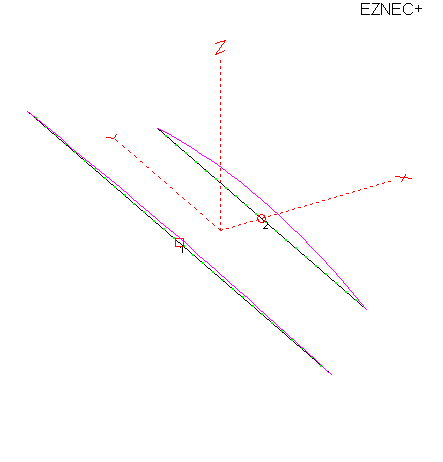
We can model antenna coupling using a program like EZNEC. With two broadside 80-meter dipoles, each 67-feet high over medium soil, with the antennas spaced 200 feet apart, we have the following receiver voltage, current, and power levels for matched receiver input, shorted receiver input, and open receiver input:
| EZNEC+ ver. 5.0 80 meter dipoles spaced 200 ft ------ Transmitter data -------- Frequency = 3.5 MHz Voltage = 288.6 V at 4.82 deg. Current = 3.478 A at 0.0 deg. Impedance = 82.67 + J 6.969 ohms Power = 1000 watts SWR (50 ohm system) = 1.672 |
EZNEC+ ver. 5.0 80 meter dipoles spaced 200 ft --------------- Receiver DATA --------------- Frequency = 3.5 MHz Voltage = 34.42 V at 39.71 deg. Current = 0.4198 A at 39.71 deg. Impedance = 82 + J 0 ohms Power = 14.45 watts Total transmitter power = 1000 watts Total receiver power = 14.45 watts |
| EZNEC+ ver. 5.0 80 meter dipoles spaced 200 ft ------ Transmitter data -------- Frequency = 3.5 MHz Voltage = 288.6 V at 4.82 deg. Current = 3.478 A at 0.0 deg. Impedance = 82.67 + J 6.969 ohms Power = 1000 watts SWR (50 ohm system) = 1.672 |
EZNEC+ ver. 5.0 80 meter dipoles spaced 200 ft ---------------Receiver short DATA --------------- Frequency = 3.5 MHz Current = 0.8329 A at 36.4 deg. Impedance = 0.001 + J 0 ohms |
| EZNEC+ ver. 5.0 80 meter dipoles spaced 200 ft
|
EZNEC+ ver. 5.0 80 meter dipoles spaced 200 ft --------------- Receiver open DATA --------------- Frequency = 3.5 MHz Voltage = 71.14 V RMS Impedance = 1E+12 + J 0 ohms |
Actual voltage and current is probably somewhere around the matched value, but the second antenna can deliver up to .83 amperes, or 100-volts peak voltage, to a receiver depending on receiver input impedance. This can cause receiver damage, even though the antennas are 200-feet apart, not very high, and horizontally polarized.
Coupled Power, very close-spaced elements, different bands
Five-foot spacing between elements
Frequency = 21 MHz
Total applied power = 1000 watts
Load on 1 (20M element)
Termination Impedance = 50 + J 0 ohms
Voltage = 50.37 V
Current = 1.007 A
Total load power = 50.74 watts
The 20 meter element looks like 155.8 +j434.7 ohms on 15 meters. In theory if we terminate that element with the conjugate, we will have maximum coupling.
Frequency = 21 MHz Total applied power = 1000 watts
Load 1 Voltage = 753.6 V
Current = 1.632 A
Impedance = 155.8 - J 434.7 ohms
Total load power = 414.9 watts
With the very same spacing and power, if the 15M termination impedance of the 20 meter element is 155.8 -j434.7, we now have 415 watts coupled power. Obviously the impedance reflected back to the 20M element is critical, yet no one to this date considers this. Not antenna manufacturers, not filter manufacturers, and not articles on filters or stubs.
Near-minimum coupling would occur when the filter/transmission line combination, on 15 meters but at the 20 meter element feedpoint, would be closest to a dead short or open with inductive reactance. Since the resistive part is 155-ohms, a 1 ohm j0 termination on 15 meters would be a 155:1 mismatch. It would be difficult to obtain 155*155= 24025 ohms on 15 without hurting 20, so a low resistance with inductive sign appears to be a better target for feeder and filter (stub) on the 20M element.
With a 20 meter open 1/2 wave stub across the 20M element, and assuming 50 j0 as the 15M load on the 20 meter element, we have:
Frequency = 21 MHz Total applied power = 1000 watts
Load 1 Voltage = 22.09 V
Current = 0.4417 A
Impedance = 50 + J 0 ohms
Total load power = 9.756 watts
With the other solution, which is a 20 meter shorted 1/4wave stub across the 20 meter feedpoint, we have:
Frequency = 21 MHz Total applied power = 1000 watts
Load 1 Voltage = 44.77 V
Current = 0.8954 A
Impedance = 50 + J 0 ohms
Total load power = 40.09 watts
These load power levels are not etched in stone, because they ASSUME the receiver looks like 50 j0 on 15 meters when the receiver is set to 20 meters. Actual receiver power will almost certainly be much less than the above cases, although it could be more with sour lengths of feed line in combination with certain receiver input impedances.
While I don't have time to look at combinations in more detail, the purpose of this is to show that nearly all stub and filter, or antenna coupling analysis on the Web and in articles, that do not consider source and load impedances, are incorrect. Electrical distance from filter or stub to the antenna and the radio system has a large effect on attenuation and coupled power. Unfortunately this distance varies with the type of filter, radio (or amplifier), or antenna. Here are some general rules:
- The stub belongs at the antenna element, and the optimum stub type and length varies with the antenna characteristics. In general (except for cases of odd-multiple resonances), a short is always best, so a high-Q series-resonant trap will likely always be better than a stub.
- If a stub is used, it is worth investigating optimum type and optimum distance from load or source.
- Coupled power is never what a 50 ohm load shows
- Heat or stress on a filter is never what a 50-ohm load test shows
- Power is largely reflected from filters and stubs, NOT absorbed
Safe Way to Test
The best way to prevent damage is to measure power from one antenna to a dummy load while the other transmitter is running at maximum power. This us an idea of the path loss between antennas. If one or both antennas are on rotors, they should be rotated for maximum signal level.
I measured my antennas with a selective level meter, and a wide-range matching network to tune for maximum power (or a load that really represents the equipment impedance). This allowed coupled power measurements at greatly reduced (safe) power levels.
I have some measurements on this page http://www.w8ji.com/coaxial_cable_leakage.htm and in the text below.
In this group of single-tower antennas, highest coupling occurs from the 15-meter antenna to the 40-meter antenna system. The 15-meter Yagi couples to the 40-meter Yagis on 15-meters with -31 dB attenuation, because the 40-meter Yagis below the 15 meter antenna is harmonically resonant on 15 meters.
With 45-foot spacing, because of impedance and resonance mismatches, there is negligible measured coupling from 40- to 20-meter antennas. This is also true for all other bands tested, because the antennas do not work well on harmonics.
This system also has potential problems from a low 80-meter dipole on this tower to a SE/NW broadside 80-meter dipole, up 160-feet on a 318-foot tower. Despite over 250-foot spacing, coupling between these two 80-meter antennas is high enough to raise concerns of receiver damage. This could happen if both antennas are used on 80-meters at the same time at high power.
Signal levels from the 160-meter vertical antennas, even with 350-feet of spacing, are also worrisome in my old high 160-meter dipole. This is mostly because my high 160-meter dipole is not directly broadside to my 160-meter verticals. Fortunately, I almost never use my transmitting antennas to receive on 160.
160-Meter Antenna Coupling
The table below lists receiver port levels and path loss between my transmitting and receiving antennas on 160-meters.
TX antennas: eight direction 4-square and 200-ft omni, with omni centered in 4-square
Reference antenna: 70-foot vertical 375 feet SW of TX antenna center point
Rear Bev: ~1500 feet SW of TX antennas
Rear Verticals: 8-cir array ~1200 feet SW of TX antennas
NE Front New: Pair of broadside 800-foot Beverages, 375 feet broadside, about 600 ft NNW of TX antenna
NE Front Bev old: pair of broadside 1200 ft beverages 300 feet NE of TX antennas
| Antenna test null system 10/26/2011 | Power at 5 watts | all levels in dBm or dB | ||||||||||||
| nflr-76 | tx ants | tx ants | tx ants | tx ants | tx ants | tx ants | tx ants | tx ants | tx ants | TX delta | MAX | MIN | ||
| rear vert | omni | N | NE | E | SE | S | SW | W | NW | |||||
| N | -26.47 | -36.37 | -39.14 | -34.12 | -37.5 | -25.4 | -22.25 | -25.15 | -34.9 | 16.89 | -22.25 | -39.14 | ||
| NE | -23.3 | -28.95 | -41 | -28.38 | -26 | -19.5 | -17.05 | -20.5 | -28.15 | 23.95 | -17.05 | -41 | ||
| E | -29.47 | -42.74 | -44.3 | -37.1 | -34.6 | -38.75 | -33.4 | -36.9 | -39.7 | 14.83 | -29.47 | -44.3 | ||
| SE | -30.9 | -40 | -51.3 | -44.8 | -42 | -30 | -28.2 | -31.4 | -41.4 | 23.1 | -28.2 | -51.3 | ||
| S | -31.15 | -38.65 | -47.8 | -50.5 | -41.8 | -28.8 | -27.65 | -31 | -41 | 22.85 | -27.65 | -50.5 | ||
| SW | -29.75 | -39.85 | -51.6 | -44.3 | -42.4 | -30 | -28.1 | -31.3 | -41.1 | 23.5 | -28.1 | -51.6 | ||
| W | -26.3 | -37.7 | -52 | -47.6 | -38.75 | -28.5 | -27.5 | -31.15 | -39.5 | 25.7 | -26.3 | -52 | ||
| NW | -32.55 | -40.15 | -51 | -53.6 | -41.9 | -30.35 | -29.5 | -32.8 | -42.8 | 24.1 | -29.5 | -53.6 | ||
| Reference | -13.8 | -20.95 | -29 | -19.8 | -21.3 | -12.5 | -9.45 | -11.8 | -19.8 | 19.55 | -9.45 | -29 | ||
| Losses | ||||||||||||||
| N vrt to ref | 12.67 | 15.42 | 10.14 | 14.32 | 16.2 | 12.9 | 12.8 | 13.35 | 15.1 | 6.06 | 16.2 | 10.14 | ||
| NE vrt to ref | 9.5 | 8 | 12 | 8.58 | 4.7 | 7 | 7.6 | 8.7 | 8.35 | 7.3 | 12 | 4.7 | ||
| E vrt to ref | 15.67 | 21.79 | 15.3 | 17.3 | 13.3 | 26.25 | 23.95 | 25.1 | 19.9 | 12.95 | 26.25 | 13.3 | ||
| SE vrt to ref | 17.1 | 19.05 | 22.3 | 25 | 20.7 | 17.5 | 18.75 | 19.6 | 21.6 | 7.9 | 25 | 17.1 | ||
| S vrt to ref | 17.35 | 17.7 | 18.8 | 30.7 | 20.5 | 16.3 | 18.2 | 19.2 | 21.2 | 14.4 | 30.7 | 16.3 | ||
| SW vrt to ref | 15.95 | 18.9 | 22.6 | 24.5 | 21.1 | 17.5 | 18.65 | 19.5 | 21.3 | 8.55 | 24.5 | 15.95 | ||
| W vrt to ref | 12.5 | 16.75 | 23 | 27.8 | 17.45 | 16 | 18.05 | 19.35 | 19.7 | 15.3 | 27.8 | 12.5 | ||
| NW vrt to ref | 18.75 | 19.2 | 22 | 33.8 | 20.6 | 17.85 | 20.05 | 21 | 23 | 15.95 | 33.8 | 17.85 | ||
| rear bev | omni | N | NE | E | SE | S | SW | W | NW | |||||
| N | -16.58 | -23 | -44.8 | -31 | -31 | -14.1 | -15.4 | -17.3 | -25.1 | 30.7 | -14.1 | -44.8 | ||
| NE | -20.75 | -26.75 | -37.9 | -31.75 | -26.3 | -17.85 | -20.7 | -24.8 | -30.5 | 20.05 | -17.85 | -37.9 | ||
| E | -28.1 | -31.7 | -40.65 | -34.7 | -30.5 | -24.9 | -30.4 | -33.7 | -36.5 | 15.75 | -24.9 | -40.65 | ||
| SE | -27.9 | -33.7 | -42.75 | -39.9 | -38.5 | -25.3 | -26.3 | -28.5 | -35.1 | 17.45 | -25.3 | -42.75 | ||
| S | -28 | -32.9 | -42.3 | -37.7 | -34.7 | -25.2 | -27 | -29.5 | -34.7 | 17.1 | -25.2 | -42.3 | ||
| SW | -24.6 | -30.7 | -34.3 | -31.8 | -30.9 | -22.5 | -21.9 | -24.5 | -29.8 | 12.4 | -21.9 | -34.3 | ||
| W | -40 | -46.7 | -49.6 | -47.9 | -51 | -38 | -37 | -39.2 | -45.3 | 14 | -37 | -51 | ||
| NW | -40 | -46.6 | -50.85 | -46.1 | -47.9 | -38.4 | -37.7 | -39.4 | -45.9 | 13.15 | -37.7 | -50.85 | ||
| Reference | -13.26 | -19 | -21.27 | -17.85 | -19.4 | -11.5 | -9.85 | -11.6 | -17.65 | 11.42 | -9.85 | -21.27 | ||
| Losses | ||||||||||||||
| N bev to ref | 3.32 | 4 | 23.53 | 13.15 | 11.6 | 2.6 | 5.55 | 5.7 | 7.45 | 20.93 | 23.53 | 2.6 | ||
| NE bev to ref | 7.49 | 7.75 | 16.63 | 13.9 | 6.9 | 6.35 | 10.85 | 13.2 | 12.85 | 10.28 | 16.63 | 6.35 | ||
| E bev to ref | 14.84 | 12.7 | 19.38 | 16.85 | 11.1 | 13.4 | 20.55 | 22.1 | 18.85 | 11 | 22.1 | 11.1 | ||
| SE bev to ref | 14.64 | 14.7 | 21.48 | 22.05 | 19.1 | 13.8 | 16.45 | 16.9 | 17.45 | 8.25 | 22.05 | 13.8 | ||
| S bev to ref | 14.74 | 13.9 | 21.03 | 19.85 | 15.3 | 13.7 | 17.15 | 17.9 | 17.05 | 7.33 | 21.03 | 13.7 | ||
| SW bev to ref | 11.34 | 11.7 | 13.03 | 13.95 | 11.5 | 11 | 12.05 | 12.9 | 12.15 | 2.95 | 13.95 | 11 | ||
| W bev to ref | 26.74 | 27.7 | 28.33 | 30.05 | 31.6 | 26.5 | 27.15 | 27.6 | 27.65 | 5.1 | 31.6 | 26.5 | ||
| NW bev to ref | 26.74 | 27.6 | 29.58 | 28.25 | 28.5 | 26.9 | 27.85 | 27.8 | 28.25 | 2.84 | 29.58 | 26.74 | ||
| Frnt Bev | omni | N | NE | E | SE | S | SW | W | NW | |||||
| NE New | -23.45 | -17.15 | -22.75 | -27.5 | -29.45 | -25 | -28.3 | -25.25 | -18.36 | 12.3 | -17.15 | -29.45 | -109 dBm | |
| NE Old | -11.93 | -11.9 | -9.82 | -10.5 | -25.4 | -19.15 | -21.1 | -16.1 | -26.1 | 16.28 | -9.82 | -26.1 | -112 dBm | |
| Reference | -13.26 | -19 | -21.27 | -17.85 | -19.4 | -11.5 | -9.85 | -11.6 | -17.65 | 11.42 | -9.85 | -21.27 | ||
| Losses | ||||||||||||||
| N bev to ref | 10.19 | -1.85 | 1.48 | 9.65 | 10.05 | 13.5 | 18.45 | 13.65 | 0.71 | 20.3 | 18.45 | -1.85 | ||
| NE bev to ref | -1.33 | -7.1 | -11.45 | -7.35 | 6 | 7.65 | 11.25 | 4.5 | 8.45 | 22.7 | 11.25 | -11.45 | ||