There are three primary types of arrays, collinear, broadside, and end fire.
Collinear describes two or more things arranged in a straight line. Extended double Zepps and two half waves in phase are examples of collinear arrays. A 5/8th wave radiator, which developes gain when placed over an infinite ground plane through ground reflection image, is also a collinear. The 5/8th wave is collinear with the ground reflection image.
Broadside is used to describe pattern in relationship to spatial area occupied by the array. While a collinear array is a broadside array, the term broadside is generally reserved for non-collinear arrangements.
End fire arrays are arrays with elements arranged in a row, running in the direction(s) of maximum radiation. Yagi antennas, W8JK arrays, and log periodic dipole arrays are all end fire arrays. They fire in the direction of the boom through the plane of the elements.
Before analyzing stacking (broadside) or collinear antennas, we really should understand how antenna systems produce gain. There is a common "Ham-myth" that doubling the number the number of elements doubles field strength (3dB more gain). This actually isn't true. Doubling the number of elements, or even doubling array size, can change gain almost any amount. While there are isolated cases where a size or element number change might result in 3db additional gain, it is through coincidence rather than science. To understand this, we have to understand what causes "gain".
When a fixed power level is coupled into an antenna, all energy not lost as heat is radiated as an electromagnetic field. This radiation is unevenly distributed in space, much like a volume of air in a rubber balloon. The creation of new or deeper nulls, in angles and directions initially having significant radiation, forces energy into narrower directions. This increases level in those areas at the expense of radiation in other direction, much like squeezing a balloon with our hands will cause a balloon to expand in certain directions at the expense of others. It is this squeezing of the radiation into a smaller spatial area that causes a "gain" increase. A newly created null or a deeper null removes energy from null areas, forcing that energy in what we hope are more useful or desirable directions. In other words, because applied transmitter power is constant, energy formerly radiated in areas of significant radiation moves to enhance field strength in other directions. This effect is not from increased element number area or physical array size. The gain increase is actually caused by redistribution of energy, because of the new, wider, or deeper null areas. When a cancellation of radiation removes power from areas with significant radiation, the pattern becomes narrower. This is an increase in directivity. When directivity increases without significantly increasing heat losses, "gain" has to increase.
Null forming is caused by the relative phase and level relationship between two or more sources of radiation at different points in space around an array. If we arrange elements over space, phasing the elements in a way that forces a null where there is very little energy, there will not be much pattern directivity or gain change. This is because the system is attempting to remove energy from an area already lacking significant energy. The reward is small, because there is little energy to redirect to more useful angles or directions. An example of this is the quad element, as height is varied. When a horizontally polarized full-wave quad element is placed 1/2λ above ground, or multiples of 1/2λ above ground, quad gain over a dipole is minimized or can even be negative. This is because the quad element is trying to force a null in an area that already has a deep null from ground reflection. Conversely, when the quad element is compared to a dipole , each at 3/4λ high (which produces a strong overhead radiation lobe from ground reflection), or if a quad element is compared to a dipole in free space, quad element gain over a dipole is maximized. This is because, under the latter conditions, the dipole had significant energy where radiation from the quad's second current maximum forces a null.
This effect is sometimes called pattern multiplication. Before antenna modeling software was commonly available, we often used pattern multiplication to estimate patterns and gain. Pattern multiplication remains a useful tool, helping us visualize why or how a particular array behaves in a certain way.
We should always consider patterns caused by spacing and phasing, including earth reflections, when planning optimum spacing. At lower heights optimum spacing will often vary as element mean height above earth, or null points created by original cells making up an array, vary. We should never assume a certain spacing always produces optimum gain, or that effective aperture somehow sets optimum broadside or collinear spacing. In fact, doubling an antenna's size almost never doubles antenna gain (3dB).
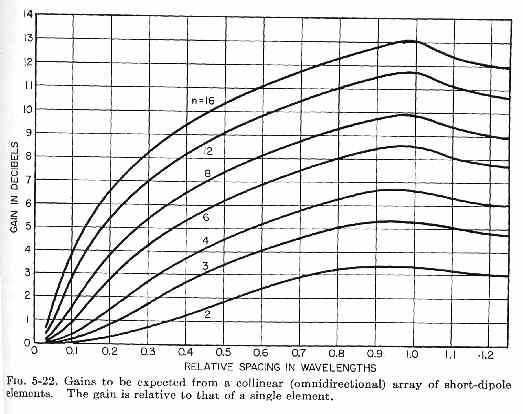
I've added graphs from Jasik's Antenna Engineering Handbook throughout this article. These graphs show theoretical maximum gain of short, lossless, dipole elements when arranged end-to-end (Collinear) or parallel above or next to each other (stacked broadside). These graphs represent the maximum possible theoretical or mathematical gain of array elements having a single current maxima at or near the center, such as a dipole or center fed 5/8th wave element.
First we have the end-to-end or collinear element placement gain.
The "Relative Spacing In Wavelengths" in the graph (fig 5-22) above is the current-maximum spacing of the elements, not element "tip" or "center" spacing.
Gain for two collinear 1/2λ (or shorter) dipole elements peaks with ~0.9λ (wavelength) spacing. Radiation is caused by current, and so areas of maximum current are where radiation primarily occurs. With a 1/2λ dipole in each element, the dipole center spacing below would be 0.9 - .25 -.25 = 0.4λ. The overall array length would be .9 + .25 + .25 = 1.4λ
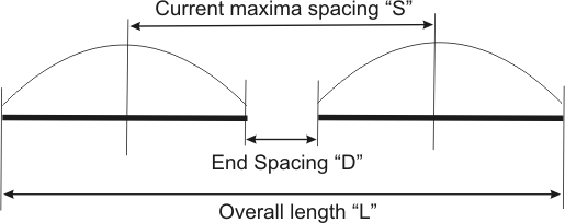
With two dipoles placed end-to-end at the center with almost no end spacing, spacing of current maximums (S) would be .25+.25=.5λ. Overall length would be twice that of a single dipole, or 1λ. Maximum theoretical gain for this spacing is found on the graph above, at the crossing of the vertical 0.5 RELATIVE SPACING IN WAVELENGTHS and intersection of "curve 2" (the two-element curve), as just under 2dB over a single element. Gain of two half waves in phase with close end-spacing is always less than 2dB over a single element in ANY collinear antenna using 1/2λ or shorter elements with very small element end spacing (D). Despite what is commonly claimed in Ham-myths, we see simply doubling the number of elements and doubling array length does not guarantee a gain increase of 3dB!
Obtaining 3dB gain by doubling the number of collinear elements from one to two requires a significant size increase over double-size. A collinear two-element antenna, using half-wave dipole elements, has 3dB gain over a single dipole when dipole current maxima spacing (S) is .75λ. This is .25λ D, or 1.25λ overall L in the case of 1/2λ dipole elements, for 3dBd gain. Keep in mind 3dB is not the maximum obtainable gain for two elements. Maximum theoretical gain is about 3.25dBd, and for 1/2λ dipole elements, occurs at about 0.9λ S current maxima spacing, or 1.45λ L overall length. If the elements were 5/8th wave, the result would actually be less gain! This gain loss occurs from the addition of areas with out-of-phase currents in the 5/8th wave element.
Doubling gain again (3dB more gain, for a total of ~6dB), over the two-element case, requires a minimum of four collinear elements. In this case array length would be 2.75λ, or 5.5 times the overall length of the initial dipole.
A four or more element collinear array can produce over 6dBd gain by a current maxima spacing over 0.75λ. If, for example, the array has 0.95λ current maxima spacings, a four element array would have an optimum gain of 6.7dB. This would result in an overall physical length of 3.35λ. Again, this does not follow the "double elements is 3dB more gain" myth. Now the gain is 6.7dBd, it has 4 (or more) times the elements, and has 6.7 times the length of the initial dipole. To obtain 6.7dB gain over a dipole, the array had to be 6.7 times the dipole length! To obtain 6 dB over a dipole, the array length had to be 5.5 times the dipole length.
The more elements the array has, the further individual elements must be spaced for optimum gain. Doubling physical size while doubling the number of elements does not double collinear gain.
EXAMPLE OF COLLINEAR
Using EZNEC, we see the gain of a lossless dipole in freespace is 2.14 dBi.
Adding a second collinear element with close end-to-end spacing, which doubles antenna size, we have:
We now have 3.71-2.14 = 1.57dBd gain. We doubled antenna size, but gain increased only 1.57 dB. Looking at Jasik's collinear gain graph, we find very close agreement. Current maximum spacing "S" in the model is 0.5λ, and maximum theoretical gain predicted in Jasik's graph is about 1.75dB:
Increasing spacing S to 0.9 wavelengths should produce maximum gain for two lossless collinear dipole elements. EZNEC shows, for full-size dipoles:
We now have 5.37-2.14 = 3.23 dBd gain. This is in close agreement with Jasik's graphs. 3dB gain increase requires 2.6 times antenna area increase, and this is with simple dipoles. Generally, as individual elements or cells (groups) of elements making up an array become more directive, optimum spacing distance increases.
When an antenna with azimuthal or compass-heading directivity increase is placed above earth, pattern multiplication and gain is not largely affected by earth. It is still possible to nearly obtain full theoretical gain at any height. This is because the earth is not trying to force a null where the array is also trying to create a null.
Broadside array usually describes elements or cells or elements placed parallel and one above the other. The graph below shows OPTIMUM or maximum possible gain, not the actual gain an array might have. The graph below is for 1/2λ dipole elements (or shorter) in freespace. Stacked Yagis would, in general, require wider spacing to produce maximum possible gain, and almost always produce less than the theoretical maximum gain increase shown below. This is because a Yagi generally has a significant null off the antenna's forward lobe. The differently located nulls, or reduced energy level in areas where dipoles normally have significant radiation, change optimum broadside stacking distance.
Optimum broadside stacking distance increases with more directive elements or cells. This is why a pair of multi-element Yagi's stacked requires wider spacing for the same gain increase than a pair of dipoles, and why less maximum stacking gain is possible with the Yagi than we might obtain with stacked dipoles. Think of it this way, if the antenna is already narrow there is less unwanted energy available to move to the main lobe. Again, this shows doubling the number of elements or size does not double the gain.
Here is the optimum gain graph for dipoles in freespace:
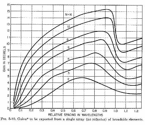
We can see maximum gain occurs at .675λ stacking height. The stacking gain is 4.8db, not 3dB as we often see claimed. Again the more elements the narrower the pattern, and the narrower the pattern the wider spacing must be between elements for maximum gain.
Here is the freespace EZNEC plot of two stacked (broadside) dipole elements:

Compared to a lossless dipole in freespace, gain is 5.96 - 2.14 = 3.82 dBd. This agrees with the graph from Jasik.
The presence of earth influences optimum stacking distance. This is because the earth is trying to force a null in the same area or areas that elevation stacking is also influencing. The earth can be considered a second element, and before computer modeling, this influence was often visualized and calculated by using fields from an imaginary "image antenna" placed down in the earth. The "image antenna" was not something that actually existed, but was a tool for calculating elevation patterns in the presence of earth. If we search old textbooks and handbooks, the image antenna often appeared.
If we have a lossless dipole at 1/2λ over perfect earth, we have this basic gain:
For a single lossless dipole, 1/2λ over perfect earth, gain is 8.4 dBi. Now let's watch when we stack the dipoles at the same 1/2λ wave stack spacing:
The system now has 10.91 - 8.4 = 2.51 dBd gain. Freespace stacking gain was 3.82 dBd, stack gain is about 1.3 dB less.
Moving the dipole to 3/4λ height, we have the following dipole pattern and gain:
This is 8.05dBi gain, now with significant energy where the stack would force a null. Adding the second broadside element, in the stack, we have:
Gain is now 11.31 dBi, or 3.26 dBd (dipole at 3/4λ).
I hope these graphs help dispel the myth that doubling number of elements, or doubling array size, doubles gain (3dB gain). Things are not that simple, and things almost never follow that rule.
1.) Doubling elements or array size does not guarantee doubling (3 dB more) gain. That's a myth, because it is almost never true.
2.) The narrower initial antenna pattern is, the wider stacking distance generally becomes for maximum gain improvement. This does, in some very rough way, relate to effective aperture.
3.) Optimum stacking distance for gain is virtually never 1/2λ, it is almost always wider.
4.) Optimum stacking distance can be very wide for arrays with multiple sharp-pattern antennas, or cells, in the array.
5.) Maximum gain occurs only when a null is forced in an area that formerly contained significant energy levels. If the original element or cell of elements has a null where the stacking distance tries to force a new null, maximum gain increase is reduced.
6.) Height above ground affects antenna pattern, and because of that, height also affects optimum stacking distance.
7.) Determining optimum stacking height or distance requires a model that includes earth, as well as feed line and conductor losses.
The optimum feed system is generally a distributed or branching type of feed system. There are many articles suggesting feed systems, so I'll only point out a few places where caution should be applied.
One error is using long lengths of 75-ohm line to co-phase two 50-ohm elements. An odd-quarter wavelength 75-ohm line transforms impedances because the line is mismatched, and has standing waves. If the line is lossless with a perfect 50 0j ohm load, the 75-ohm SWR all along the 75-ohm line is 1.5:1. This means, at odd-quarter wave distances, line impedance becomes 1.5*75 = 112.5 0j ohms. Two of those impedances in parallel are 56.25 ohms. Unfortunately, the required coaxial cable physical length means elements must ether be less than 1/2λ apart, or we must use longer feed lines from the Q-sections to element centers.
Many articles make the Q-section longer than λ/4, such as 3λ/4 or 5λ/4. We should be careful doing this, for two reasons:
Consider the case of a line 5λ/4 wavelengths long. Such a line has five 90-degree sections in series. If frequency changes 2%, it causes a 2% error in each λ/4 section. Errors in each of the five sections add, and now the total line error is 10%. The Q-section not only has additional loss, it also has reduced bandwidth.
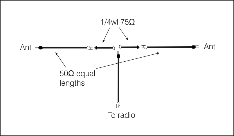
Using a 50-ohm section from each element to its respective Q-section, so each Q section only needs to be λ/4 long, will always increase bandwidth and often decrease losses. It is also not difficult to implement. My 6-meter Yagi stack uses 50-ohm equal length lines to the Q-sections, which are only λ/4 long. Length of the 50-ohm sections does not matter, so long as they are equal, because the 50-ohm sections are matched, and essentially have a 1:1 VSWR. If I make a velocity factor error, or change frequency, or have 75-ohm line losses, errors and/or problems are 5 times less!
I'm not forced to have feed lines between the antennas that can only be changed in multiples of λ/2, such as λ/4, 3λ/4, 5λ/4, and so on. I can use two equal length 50-ohm feed lines that are any physical length that reaches, with the only attention to detail the quarter wavelength 75-ohm Q-sections. This greatly reduces cable cutting errors because the long lines are matched, and only need to be equal lengths of the same cable stock.
We use broadside stacking and collinear gain most effectively in Curtain Arrays like the Lazy H antenna. You can read more about Curtain Antenna Arrays on my Sterba Curtain Lazy-H antenna page.
Unless we remove energy from an area that had significant energy, antennas cannot produce gain. If an antenna has a wide area with no radiation at all, and we designed a system to force a null totally within that same area, there would be no gain at all. The pattern must be narrowed to increase gain, and it must be narrowed in a way that does not increase heat losses faster than it concentrates electromagnetic radiation.
Earth focuses energy in the elevation plane, creating one or more nulls in elevation pattern. Height above earth, as well as quality of earth, controls the nulls formed by earth reflections. For somewhat flat earth, nulls formed by the presence of earth are all in the elevation plane of the pattern. In most cases, azimuthal beamwidth, or compass directivity, is largely unaffected by antenna height. For this reason, azimuth pattern multiplication, or gain increase by focusing in what we consider "compass direction", is largely unaffected by height above earth or changes in stacking spacing. We saw this above in the relationships between actual gain with height or vertical spacing of the antenna or antennas, and gain changes with changes in horizontal spacing or area occupied by the antenna elements.